9.5 Additional Information and Full Hypothesis Test Examples (Proportions)

HYPOTHESIS TESTING WITH ONE SAMPLE FOR PROPORTION

If a claim is made about a population proportion, we can obtain a representative sample to test the claim. Like always, we’ll start our hypothesis test by assuming the equality in the null hypothesis is true. This null assumption gives us a value for the population proportion. We know that due to sampling variability, sample statistics (in this case sample proportion [latex]\hat p[/latex] for samples of the same size drawn from a population are going to naturally vary from one sample to another. Due to this natural variation, our sample proportion is also likely going to be different from the actual proportion in the population that our sample came from. For that population, we have assumed the population proportion is the same as that in the null hypothesis. So the question is whether this difference between our sample proportion and the null parameter is due to random chance or something else.

Hypothesis testing gives us a way to find out how likely are we to observe the difference between our sample statistic and the null parameter due to random chance alone as a result of sampling variability. To investigate this, we’ll utilize the sampling distribution of sample proportions [latex]\hat p[/latex] derived from central limit theorem (CLT). Recall that if [latex]np > 5[/latex] and [latex]nq > 5[/latex], the sampling distribution of sample proportions, [latex]\hat p[/latex], will be approximately normal. Since the CLT gives us the mean and the standard error of the sampling distribution, we can use that distribution information to determine the probability of observing the difference between our sample proportion and the null parameter. This probability tells us how usual or unusual it is for us to observe a difference between our sample proportion and the proportion from the null hypothesis. If our sample is very unusual, then we have a reason doubt that the difference between our sample proportion and the null parameter is due to chance alone because we expect our carefully chosen, representative sample to be more likely usual than unusual as we expect about 95% of the sample statistics to be within two standard errors of the center of the distribution. Because we expect our sample to be usual, if our sample turns out to be highly unusual, then we’re going to reject the assumption that we made in the first place, that the null hypothesis is true, and we’re going to side with the alternative hypothesis.

Symbols used in hypothesis testing for proportions

HYPOTHESIS TESTING FOR PROPORTION STEPS

STEP 1: Write the claim (or what’s being tested) using mathematical symbols

STEP 2: Write the opposite of the claim using mathematical symbols

STEP 3: Write the null and alternative hypothesis

STEP 4: Identify the tail-type of the test and the level of significance, [latex]\alpha[/latex]. If [latex]\alpha[/latex] is not given, assume it to be 5% or 0.05.

STEP 5: Check if CLT conditions are valid: [latex]np > 5[/latex] and [latex]nq > 5[/latex] .
Assume the equality in the null hypothesis is true. Using the population proportion, [latex]p[/latex], from the null hypothesis, draw a sampling distribution of sample proportions. Record the center and the standard deviation of the sampling distribution.

\[\mu_{\hat p}=p\]

\[\sigma_{\hat p}=\sqrt{p(1-p)\over n}\]

STEP 6: On the horizontal axis of the graph from STEP 5, record the position of your sample proportion, [latex]\hat p[/latex]. For one-tailed tests, the area to the tail from this [latex]\hat p[/latex]  is the [latex]p[/latex]-value. For two-tailed test, [latex]p[/latex]-value is the double of the that tail area.

STEP 7: Make the decision by comparing [latex]p[/latex] -value with [latex]\alpha[/latex].

• If [latex]p[/latex]-value [latex]< \alpha[/latex], ⇒ reject [latex]H_0[/latex] Test results are statistically significant and sample data provides enough evidence to support the alternative hypothesis, [latex]H_a[/latex]
• If [latex]p[/latex]-value [latex]\ge \alpha[/latex], ⇒ Fail to reject [latex]H_0[/latex]
  There’s not enough evidence to support [latex]H_a[/latex]

STEP 8: Interpret your decision in the context of original claim.

EXAMPLE

A study by Gallop Poll reports that 40% of Americans fear public speaking. A student believes that less than 40% of students at her school fear public speaking. She randomly surveys 361 schoolmates and finds that 135 report they fear public speaking. Conduct a hypothesis test to determine if the percent at her school is less than 40%.

SHOW SOLUTION

Is the claim about a population mean or proportion?
How can we tell?

The student’s claim here is about the percent of students at her school who fear public speaking (which she believes is less than 40%). The information she’ll need to gather from each person in her sample is whether they fear public speaking or not. This will be categorical data. She can calculate what percent (proportion) of the people in her sample with the categorical data. With a sample proportion, she can test claims made about a population proportion. Since she doesn’t know the exact percent of students at her school who fear public speaking, let’s call this unknown percentage (proportion) [latex]p[/latex].

[latex]p[/latex] = proportion of students at her school who fear public speaking

Sample information
Sample size, [latex]n = 361[/latex]
Number of successes, [latex]x = 135[/latex]
Sample proportion, [latex]\hat p = 135/361[/latex]

STEP 1: Write the claim (or what’s being tested) using mathematical symbols

Claim:	The percent of students at her school who fear public speaking	is less than	40%
	[latex]p[/latex]	[latex]<[/latex]	[latex]0.40[/latex]

STEP 2: Write the opposite of the claim using mathematical symbols
Opposite of the claim: p ≥ 0.40

STEP 3: Write the null and alternative hypothesis
The null hypothesis is the statement that contains the condition of equality which in this case is the opposite of the claim

[latex]H_0: p \ge 0.40[/latex] [latex]H_a: p < 0.40[/latex]

OR

[latex]H_0: p = 0.40[/latex] [latex]H_a: p < 0.40[/latex]

 

STEP 4: Identify the tail-type of the test and the level of significance, α. If α is not given, assume it to be 5% or 0.05.
This is a left tailed test. Why?
Since the level of significance is not given, we’ll assume it to be 5%. That is, [latex]\alpha = 0.05[/latex]

STEP 5: Check if CLT conditions are valid: [latex]np > 5[/latex] and [latex]nq > 5[/latex].
This is the stage where we assume the equality in the null hypothesis is true, that is, assume p = 0.40. Note that p is the proportion of students at her school who fear public speaking. We’re assuming that there’s no difference between her school and the Gallup Poll results for the proportion of those who fear public speaking.
[latex]np = (361)(0.40) = 144.4[/latex] and [latex]nq = n(1– p) = 361(1– 0.40) = 216.6[/latex]. Since both are more than 5, we know that the sampling distribution of sample proportion will be approximately normally distributed with mean of [latex]\mu_{\hat p}[/latex], and standard deviation (also known as standard error) of [latex]\sigma_{\hat p}[/latex]. \[\mu_{\hat p}=p=0.40\]

\[\sigma_{\hat p}=\sqrt{\frac{p(1-p)}{n}}=\sqrt{\frac{0.40(1-0.40)}{361}}=0.0257841025556\]

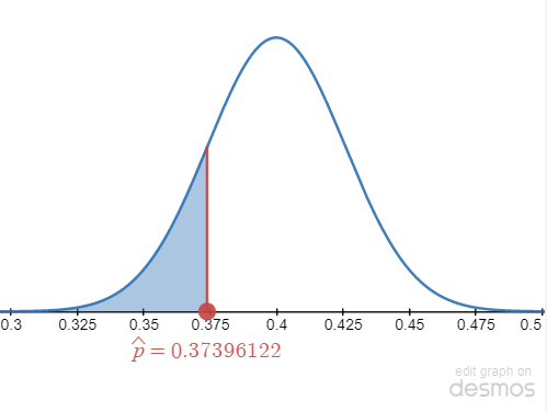
STEP 6: Plot [latex]\hat p[/latex] and find the p-value.
[latex]\hat p[/latex] is plotted on the graph above. Since the test is left-tailed, the p-value is the area to the tail from [latex]\hat p[/latex], shaded in blue on the graph above. Let’s use an online calculator such as DEMOS or STATKEY to find the  p-value, which is going to be the left tail area.

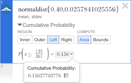
DESMOS

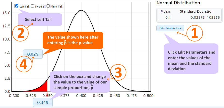
STATKEY

On StatKey main page, click on Theoretical Distributions, then Normal
1) Click on Edit parameters on the right and enter the mean as 0.40 and standard deviation as 0.025784102556
2) Select Left Tail checkbox on the top left of the graph
3) Change the value to that of our sample statistic, [latex]hat p = 135/361 = 0.374[/latex] (3 decimal places)
4) The value shown in this box at this stage is the p-value

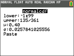
Ti-83/84+

Enter the following, select Paste and press the ENTER button twice.

STEP 7: Make the decision by comparing p-value with α
[latex]p[/latex]-value is 0.156277027764 which is greater than α of 5%. Since [latex]p[/latex] -value is greater than α, we fail to reject the null hypothesis ⇒ There’s not enough evidence to support Ha.

STEP 8: Interpret your decision in the context of original claim
There is insufficient evidence to support the claim that less than 40% of students at the school fear public speaking.

 

ONLINE CALCULATOR Approach

SUBEDI Calculator

Go to Inference for the Proportion @ rsubedi.com

Number of Samples

✅ ONE SAMPLE

🔲 TWO SAMPLES

Enter the null proportion
[latex]p_o: \fbox{$\mathstrut\;0.40\;$}[/latex]

Alternative Hypothesis

✅[latex]\quad\lt[/latex]

🔲[latex]\quad\gt[/latex]

🔲[latex]\quad\ne[/latex]

Confidence Interval? ← Optional

🔲 Include

Sample Statistics Information:

✅ Successes

🔲 [latex]\enspace\hat p[/latex]

Sample Size, n:
361   

Successes, x
135

CALCULATE
Results show in a panel to the right. Test statistic z, p-value, and sample proportion [latex]\hat p[/latex] are displayed.

LibreText Calculator

Go to: Hypothesis Test for a Proportion from the list of online calculators

Enter the following values and press Calculate.

[latex]n: \boxed{\mathstrut\;361\;}[/latex]

[latex]x: \boxed{\mathstrut\;135\;}[/latex]

[latex]p_0: \boxed{\mathstrut\;0.40\;}[/latex] ← Null value

🔘[latex]\quad\lt[/latex]

⭕[latex]\quad\gt[/latex]

⭕[latex]\quad\ne[/latex]

CALCULATE

Results displayed are:

[latex]z[/latex]: test statistic
[latex]p[/latex]: p-value