
9.5 Additional Information and Full Hypothesis Test Examples (Means)
Hypothesis Testing for MEANS
HYPOTHESIS TESTING WITH ONE SAMPLE FOR A MEAN
In the same manner as in the case with proportions, if a claim is made about a population mean, we can obtain a representative sample to test the claim. As always, we'll start our hypothesis test by assuming the equality in the null hypothesis is true. This null assumption gives us a value for the population mean. We know that due to sampling variability, sample statistics (in this case sample mean [latex]\mu[/latex] for samples of the same size drawn from a population are going to naturally vary from one sample to another. Due to this natural variation, our sample mean is also likely going to be different from the actual mean of the population that our sample came from. For that population, we have assumed the population mean is the same as that in the null hypothesis. So the question is whether this difference between our sample mean and the null parameter is due to random chance or something else.
Hypothesis testing gives us a way to find out how likely are we to observe the difference between our sample statistic and the null parameter due to random chance alone as a result of sampling variability. To investigate this, we'll utilize the sampling distribution of sample means, [latex]\bar x[/latex], derived from central limit theorem (CLT). Recall that if the sample size [latex]n\ge30[/latex] or if the population we sampled from is already normally distributed, then the sampling distribution of sample means, [latex]\bar x[/latex], will be (approximately) normal. Since the CLT gives us the mean and the standard error of the sampling distribution, we can use that distribution information to determine the probability of observing the difference between our sample mean and the null parameter. This probability tells us how usual or unusual it is for us to observe a difference between our sample mean and the mean from the null hypothesis. If our sample is very unusual, then we have a reason to doubt that the difference between our sample mean and the null parameter is due to chance alone because we expect our carefully chosen, representative sample to be more likely usual than unusual as we expect about 95% of the sample statistics to be within two standard errors of the center of the distribution. Because we expect our sample to be usual, if our sample turns out to be highly unusual, then we're going to reject the assumption that we made in the first place, that the null hypothesis is true, and we're going to side with the alternative hypothesis.
Symbols used in hypothesis testing for means
|
Population [latex]\mu[/latex] = population mean [latex]\sigma[/latex] = population standard deviation |
||
|
|||
HYPOTHESIS TESTING FOR MEAN STEPS
STEP 1: Write the claim (or what's being tested) using mathematical symbols
STEP 2: Write the opposite of the claim using mathematical symbols
STEP 3: Write the null and alternative hypothesis
STEP 4: Identify the tail-type of the test and the level of significance, [latex]\alpha[/latex]. If [latex]\alpha[/latex] is not given, assume it to be 5% or 0.05.
STEP 5: Check if CLT conditions are valid: (1) sample size [latex]n\ge30[/latex] or (2) population normally distributed
Assume the equality in the null hypothesis is true. Using the population mean [latex]\mu[/latex] from the null hypothesis, draw a sampling distribution of sample means. Record the center and the standard deviation of the sampling distribution.
\[\mu_{\bar x} = \mu\]
\[\sigma_{\bar x} = \frac{\sigma}{n}\]
STEP 6: On the horizontal axis of the graph from STEP 5, record the position of your sample mean, [latex]\bar x[/latex]. For one-tailed tests, the area to the tail from this [latex]\bar x[/latex] is the [latex]p[/latex]-value. For two-tailed test, [latex]p[/latex]-value is the double of the that tail area.
STEP 7: Make the decision by comparing [latex]p[/latex] -value with [latex]\alpha[/latex]
- If [latex]p[/latex]-value [latex]< \alpha[/latex], ⇒ reject [latex]H_0[/latex] Test results are statistically significant and sample data provides enough evidence to support the alternative hypothesis, [latex]H_a[/latex]
- If [latex]p[/latex]-value [latex]\ge \alpha[/latex], ⇒ Fail to reject [latex]H_0[/latex]
There's not enough evidence to support [latex]H_a[/latex]
STEP 8: Interpret your decision in the context of original claim.
Practice
WORKED OUT EXAMPLE - One Sample Mean
According to the Carnegie unit system, the recommended number of hours students should study per unit is 2. Are statistics students' study hours more than the recommended number of hours per unit? The data show the results of a survey of 15 statistics students who were asked how many hours per unit they studied. Assume a normal distribution for the population.
3.9, 2.1, 3.2, 1.3, 4.3, 2.4, 2.8, 3.8, 2.6, 1.6, 1, 3.9, 1.5, 2.9, 2.1
SHOW SOLUTION
How can we tell?
Since there's only one group (statistics students) involved here, and the numerical samples are taken from that group, this is the case of one sample test for the mean. Remember that to compute an average (or mean), we need numerical data, which we have here. The statement we're testing here is whether statistics students' study for more than the recommended number of hours per unit. Since the sample data provided is provided is numerical, we can calculate the sample mean, [latex]\bar x[/latex] and the sample standard deviation, [latex]s[/latex]. With this information from the sample, we can test claims made about the population mean (the average hours of study for statistics students in general). Since we don't know the exact mean of the hours of study for all statistics students, let's call this unknown mean [latex]\mu[/latex].
[latex]\mu[/latex] = mean of statistics students' study hours in general
[latex]\mu[/latex] = mean of statistics students' study hours in general
Since the population standard deviation is unknown, we'll be using a t-distribution to test our hypotheses.
Sample information
Sample data is provided: [latex]3.9, 2.1, 3.2, 1.3, 4.3, 2.4, 2.8, 3.8, 2.6, 1.6, 1, 3.9, 1.5, 2.9, 2.1[/latex]
STEP 1: Write the claim (or what's being tested) using mathematical symbols
| Claim: | mean of study hours for statistics students in general | is more than | recommended number of hours |
| [latex]\mu[/latex] | [latex]>[/latex] | [latex]2[/latex] |
STEP 2: Write the opposite of the claim using mathematical symbols
Opposite of the claim: [latex]\mu\le2[/latex]
STEP 3: Write the null and alternative hypothesis
The null hypothesis is the statement that contains the condition of equality which in this case is the opposite of the claim
| [latex]H_0:\mu\le2[/latex] [latex]H_a:\mu > 2[/latex] |
OR | [latex]H_0:\mu=2[/latex] [latex]H_a:\mu> 2[/latex] |
STEP 4: Identify the tail-type of the test and the level of significance, α. If α is not given, assume it to be 5% or 0.05.
This is a right tailed test. Why?
Since the level of significance is not given, we'll assume it to be 5%. That is, [latex]\alpha = 0.05[/latex]
STEP 5: Check if CLT conditions are valid:
Our sample size [latex]n=15[/latex] which clearly isn't at least 30. Therefore we need to make sure that our population is normally distributed before we can proceed. Fortunately, that's exactly what we're about the population in the question that it is distributed normally. Next, this is the stage where we assume the equality in the null hypothesis is true, that is, assume [latex]\mu=2[/latex]. Note that [latex]\mu[/latex] is the mean of study hours for statistics students in general. Here, by saying [latex]\mu=2[/latex], we're assuming that there's no difference between the mean of study hours for statistics students in general and the recommended number of hours per unit, that they are the same. From the central limit theorem, we know that the sampling distribution of sample means will be distributed normally with mean [latex]\mu[/latex] and standard deviation (a.k.a. standard error) given by [latex]\sigma_{\bar x}={s\over\sqrt{n}}.[/latex] Here, the test statistic [latex]t[/latex] follows a [latex]t[/latex]-distribution with [latex]n-1 = 15-1=14[/latex] degrees of freedom. The test statistic [latex]t={{\bar x - \mu}\over{s\over\sqrt{n}}}[/latex]. Let's see that on a graph:
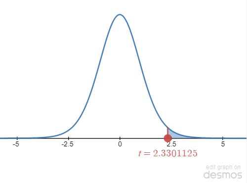
STEP 6: Plot [latex]\bar x[/latex] and find the p-value.
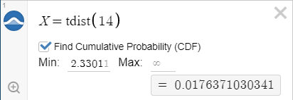
[latex]\bar x[/latex] is plotted on the graph above. Since the test is right-tailed, the p-value is the area to the tail from [latex]\bar x[/latex], shaded in blue on the graph above. Let's use an online calculator such as DEMOS or STATKEY to find the p-value, which is going to be the left tail area.
DESMOS
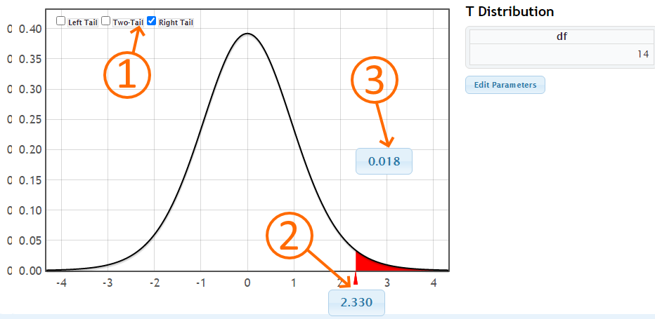
STATKEY
1) Click on Edit parameters on the right and enter the degrees of freedom
2) Select Right Tail checkbox on the top left of the graph
3) Change the value to that of our test statistic, t = 2.330 (Round t to three decimals
4) The value shown in this box at this stage is the p-value
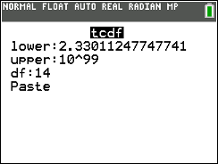
Ti-83/84+
STEP 7: Make the decision by comparing p-value with α
p-value is 0.01763710303507593 which is less than [latex]\alpha[/latex] of 5%. Since p-value is less than [latex]\alpha[/latex] , we reject the null hypothesis ⇒ There's enough evidence to support Ha.
STEP 8: Interpret your decision in the context of original claim
There is sufficient evidence to support that the statistics students study for more than the recommended 2 hours per unit. In other words, the data suggest the population mean is significantly more than 2 at [latex]\alpha = 0.05[/latex], so there is sufficient evidence to conclude that the population mean study time per unit for statistics students is more than 2.
ADDITIONAL STEPS: Interpreting p-value and the level of significance in the context of this question scenario.
Assuming the null is true
If the population mean study time per unit for statistics students is 2
If we obtain another sample using the same procedure as the original one
if you survey another 15 statistics students
There would be a 1.76 % chance
p - value(0.01763710303507593)
Find the new sample statistic (mean) to be as unusual as ours or more unusual
the sample mean for these 15 statistics students would be greater than 2.627
Significance level is equal to the probability of committing type I error, which occurs when we reject a true null hypothesis. Any study that tests the null with the same sample size with identical procedures will see a rejection rate of [latex]\alpha[/latex]. Recall that for hypothesis tests, we assume the null to be true (in reality we don't know whether it is true or not). Type I error happens when the sample data provide evidence against the null leading us to reject the null hypothesis, which in reality turns out to be true (we simply didn't know that). Note that if we reject the null, then we support the alternative. That means if we falsely reject the null, we falsely conclude that the alternative is true.
Putting it together
If
the population mean study time per unit for statistics students is 2
assume the null is true
and if
you survey another 15 statistics students
testing under identical procedures
then there would be a 5% chance
[latex]\alpha-[/latex]level
that we would end up
falsely concluding that the population mean study time per unit for statistics students is more than 2.
commit type I error
ONLINE CALCULATOR Approach
SUBEDI Calculator
Go to Inference for the Mean @ rsubedi.com
Input Type
Number of Samples
Enter the null hypothesis mean
[latex]\mu_0 = \boxed{\mathstrut \;2\;}[/latex]
Distribution Type for Test
Alternative Hypothesis
Confidence Interval? ← Optional
Enter Sample Data
Enter your data for the sample in the spreadsheet column shown. You can copy your data from the original source (comma or separated list, spreadsheet data, etc.) and paste that into the table on the calculator.
CALCULATE
Results show in a panel to the right. Test statistic t, p-value, and df. For paired data, the spreadsheet displays an additional column for the pair-wise difference of the sample data.
LibreText Calculator
Go to: Hypothesis Test for a Mean with Data from the list of online calculators
Enter the following values and press Calculate.
| Data: [latex]\boxed{\mathstrut\;3.9,2.1,3.2,1.3,4.3,2.4,2.8,3.8,2.6,1.6,1,3.9,1.5,2.9,2.1\;}[/latex] Note: Separate values with a comma. No comma after the last value. |
||
| [latex]\sigma:[/latex] Leave blank for t-test |
⭕[latex]\quad\lt[/latex]
🔘[latex]\quad\gt[/latex]
⭕[latex]\quad\ne[/latex]
|
[latex]\mu_0: \boxed{\mathstrut\;2\;}[/latex] ← Null value |
CALCULATE
Results displayed are:
[latex]s[/latex]: sample standard deviation
[latex]t[/latex]: test statistic
[latex]p[/latex]: p-value
Practice
