
6.1 The Standard Normal Distribution
The normal distribution is an extremely important distribution in statistics. When graphing naturally occurring data from many real life scenarios, the shape of the data distribution takes a bell-shaped symmetric form.
What is a distribution?
Introduction to the Normal Distribution
The curve enveloping the histogram is called a normal curve. It is bell-shaped, symmetric about the center. As a symmetric graph, note that the mean, median, and mode are all at the center as well.
Notation
[latex]X \sim N(\mu, \sigma)[/latex] means that the random variable [latex]X[/latex] is normally distributed with mean of [latex]\mu[/latex] and standard deviation [latex]\sigma[/latex].
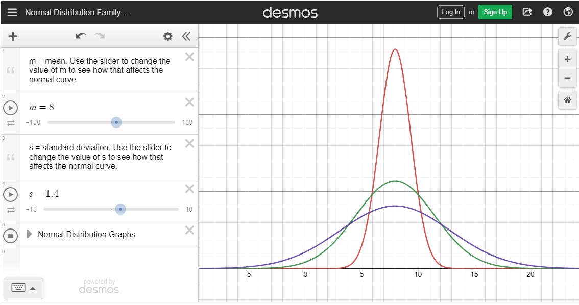
DESMOS DEMO
Use the Desmos Demo to explore the effects of changing the mean and standard deviation on the shape and center of normal distributions.
Properties of the Normal Curve
- The curve has inflection points, the points where the graph changes curvature, at exactly one standard deviation from the mean.
- The total area under the curve is equal to 100% (or 1 in decimal).
- The area under the curve to the left of the mean is equal to the area under the curve to the right of mean, which equals 0.5.
- The graph tails off towards the horizontal axis on the left and right. The x-axis is the horizontal asymptote.
What makes a distribution NORMAL?
Recall from UNIT 2 ...
In Unit 2, we explored z-scores as well as the Empirical Rule for bell-shaped distributions. We'll look at these bell-shaped distributions, more specifically, normal distributions in this unit.
Probability and Normal Distributions
Since the total area under the normal curve equals 1, and its horizontal axis represents all possible outcomes of the random variable whose distribution is represented by the normal curve, we can think of the areas under the curve as probabilities.
This is easier to comprehend if we look at a more familiar shape than the normal curve. Let's say we have a sandbox in the shape of a square of side 3 feet in a playground. A child randomly tosses a ball into the sandbox from a distance. Let's assume that the child is equally likely to hit any place inside the sandbox and will never miss the sandbox.
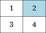
If we divide the sandbox into 4 quarters and label them 1, 2, 3, and 4 as follows, what are the chances (or what is the probability) that the child will hit the quarter 2? Since the area shaded is 25% of the total, we're going to say the chances are 25% or 0.25.
If we observe the child play this game all day, we'd expect 25% of the tosses to land in the quarter labeled 2. That is the proportion of the observations landing in quarter 2 will be 0.25. Similarly, under the normal curve as well, we can say that since the mean is at the center (under the peak), if we randomly select a value of the random variable whose distribution is normal, we'll see that there's a 50% chance that it will be below the mean and the same chance for it being above the mean.
In general, the area under the normal curve over some interval represents the probability (or the chances) of observing those values of the random variable in that interval. It is also the proportion of the outcomes of the random variable that are expected to be in that interval. When we want to calculate probabilities for a given interval, say (3, 6), the area will be different depending on the mean and the standard deviation of the normal distribution. Instead of having to deal with infinitely many normal distributions, statisticians, especially before technology became ubiquitous, simply transformed the given normal distribution to a standard normal distribution and computed the appropriate area from the standard normal distribution using standard normal or z-tables.
The Standard Normal Distribution
The standard normal distribution is a normal distribution of standardized values called z-scores. Note that z-scores answers the question: How many standard deviations away from the mean is this given data? z-scores are measured in units of the standard deviation. For any normal distribution, the z-score tells you how many standard deviations a value x is above (to the right of) or below (to the left of) the mean, [latex]\mu[/latex]. Values of x that are larger than the mean have positive z-scores, and values of x that are smaller than the mean have negative z-scores. The z-score of the mean [latex]\mu[/latex] is 0. No matter what the mean and the standard deviations are for a normal distribution, we can always talk about that normal distribution in terms of how many standard deviations away from their mean is any given x value. This leads us to the standard normal distribution, which has a mean of 0 and standard deviation of 1. We can transform a normal distribution with any mean, [latex]\mu[/latex], and any positive standard deviation, [latex]\sigma[/latex], into a standard normal distribution with the z-score formula: \[z=\frac{x-\mu}{\sigma}.\]Standard Normal Distribution is also known as the [latex]z-[/latex]distribution: [latex]Z \sim N(0,1)[/latex].
Standard Normal Distribution Probability Calculations
There are going to be two types of calculations/operations we will need to be familiar with when working with probabilities and normal distributions.
- Find AREA/PROBABILITY given VALUE
Given [latex]z-[/latex]score , find the associated probability (area) - Find VALUE given AREA/PROBABILITY
Given a probability (an area), find the [latex]z-[/latex]score
EXAMPLE
Find AREA/PROBABILITY given VALUE
For the standard normal variable [latex]Z[/latex], find the following probabilities:
- [latex]P(z\le 1.74)[/latex].
- [latex]P(z\gt -2.48)[/latex].
- [latex]P(-2.37 \le z \le 1.02)[/latex].
SHOW SOLUTION
 DESMOS CALCULATOR
Calculator Usage Guide
Click on the ▶ Cumulative Probability to open the inputs panel.
Click on the ▶ Cumulative Probability to open the inputs panel.
Click on the ▶ Cumulative Probability to open the inputs panel.
EXAMPLE
Find VALUE given AREA/PROBABILITY
For the standard normal variable [latex]Z[/latex], find the following:
- Find the z-score that separates the top 10% of the area.
- Find the z-score corresponding to the 90th percentile.
- Find the z-scores that separate the middle 95% of the area.
SHOW SOLUTION
DESMOS CALCULATOR
Calculator Usage Guide
1. Find the z-score that separates the top 10% of the area.
\[P(x \gt \colorbox{#cccccc}{$\;1.282\;\vcenter{\tiny{▾}}\;$}) =\colorbox{#ccffcc} {$\;0.10\;$} \]
z-score [latex]=1.28155156554[/latex]
2. Find the z-score corresponding to the 90th percentile.
Click on the ▶ Cumulative Probability to open the inputs panel. Select Left for the REGION and Bounds for COMPUTE, then enter 0.90 after the [latex]=[/latex] sign in the probability expression:
\[P(x \le \colorbox{#cccccc}{$\;1.282\;\vcenter{\tiny{▾}}\;$}) =\colorbox{#ccffcc} {$\;0.90\;$} \]
z-score [latex]=1.28155156554[/latex]
Same answer as above. Why?
The standard normal distribution is symmetric around its mean of zero, so it has the same shape on both sides of the mean. Due to this symmetry, the two z-scores that enclose the middle 95% are the same distance from zero but in opposite directions—one negative z-score on the left and one positive on the right.
Click on the ▶ Cumulative Probability to open the inputs panel.
Select Inner for the REGION and Bounds for COMPUTE, then enter 0.90 after the [latex]=[/latex] sign in the probability expression:
z-scores [latex]=\pm 1.95996398454[/latex]
Practice
