
12.3 The Regression Equation
Linear Regression
The regression line (also called the least squares line or the line of best fit) is derived using a procedure that minimizes the squares of the residuals (errors), which are the deviations of the observed data from the model line. The regression line has the equation: \[\hat y=a+bx\] where [latex]a=\bar y - b\bar x[/latex] and [latex]b=\dfrac{\Sigma (x - \bar x)(y - \bar y)}{\Sigma (x - \bar x)^2}[/latex].
The sample means of the [latex]x[/latex] values and the [latex]y[/latex] values are [latex]\bar x[/latex] and [latex]\bar y[/latex], respectively. The best fit line always passes through the point [latex](\bar x, \bar y)[/latex].
Remember, it is always important to plot a scatterplot first! If the scatterplot indicates that there is a linear relationship between the variables, then it is reasonable to use a regression equation to model the data.
Regressions on Desmos
The Regression Line on a Ti Calculator
The Correlation Coefficient, [latex]r[/latex]
The correlation coefficient, r is a numerical measure of strength and direction of the linear association between two quantitative variables. The formula for r is looks formidable, but once again, we'll be using technology to calculate the correlation coefficient.
If you suspect a linear relationship between x and y, then r can measure how strong the linear relationship is between the two variables.
Linear Correlation
Correlation and Regression Using StatKey
What the VALUE of [latex]r[/latex] tells us:
- The value of [latex]r[/latex] is always between –1 and +1: [latex]–1 \le r \le 1[/latex]
- The size of the correlation [latex]r[/latex] indicates the strength of the linear relationship between [latex]x[/latex] and [latex]y[/latex]
- Values of [latex]r[/latex] close to [latex]–1[/latex] or to [latex]+1[/latex] indicate a stronger linear relationship between [latex]x[/latex] and [latex]y[/latex]
- If [latex]r = 0[/latex] there is likely no linear correlation. It is important to view the scatterplot, however, because data that exhibit a curved or horizontal pattern may have a correlation of [latex]0[/latex]
- If [latex]r = 1[/latex], there is perfect positive correlation. If [latex]r = –1[/latex], there is perfect negative correlation. In both these cases, all of the original data points lie on a straight line. Of course, in the real world, this will not generally happen
The Coefficient of Determination, [latex]r^2[/latex]
The variable [latex]r^2[/latex] is called the coefficient of determination and is the square of the correlation coefficient for linear regressions. It is usually stated as a percent. It has an interpretation in the context of the data:
- [latex]r^2[/latex] , when expressed as a percent, represents the percent of variation in the dependent (predicted) variable [latex]y[/latex] that can be explained by variation in the independent (explanatory) variable [latex]x[/latex] using the regression (best-fit) line.
- [latex]1 – r^2[/latex], when expressed as a percentage, represents the percent of variation in [latex]y[/latex] that is NOT explained by variation in [latex]x[/latex] using the regression line. This can be seen as the scattering of the observed data points about the regression line.
EXAMPLE
An organization collects information on the fertility rate (children per woman) in the country and the life expectancy of a person (in years) in each country. The data for some randomly selected countries for the year 2018 are in the table below.
| Fertility rate (children per woman) | Average life expectancy (years) |
|---|---|
| 1.9 | 78 |
| 1 | 78 |
| 1 | 82 |
| 2.9 | 77 |
| 5.7 | 56 |
| 5.7 | 62 |
| 5.6 | 62 |
| 4.5 | 68 |
| 2.4 | 79 |
| 4.1 | 67 |
- 1. Use linear regression to find the equation for the linear function that best fits this data. Write your final answer as an equation in the form: [latex]y = mx+b[/latex]
- What is the value of the correlation coefficient, [latex]r[/latex]?
- Describe the strength and direction of the correlation between average life expectancy in a country and the country's fertility rate.
- What percent of the variation in the average life expectancy in a country is explained by the variation in the country's fertility rate?
- Use the model to estimate the average life expectancy in a country if the country's fertility rate is 3.6 children per woman.
- According to the model, what is the fertility rate in a country if the country's average life expectancy is 74 years?
SHOW SOLUTION
First we need to identify the independent [latex]x[/latex] and dependent [latex]y[/latex] variables. Does fertility rate depend on average life expectancy or the average life expectancy depends on the fertility rate? Reading the question, we see that we've been asked to find the percent of the variation in the average life expectancy in a country is explained by the variation in the country's fertility rate. This indicates that the fertility rate is the explanatory (independent) the average life expectancy is the response (dependent) variable. So the first column is [latex]x[/latex] and the second column in [latex]y[/latex].
WARNING! Just because a column of data appears first doesn't automatically mean that it's the independent (explanatory), x variable.
 DESMOS CALCULATOR
Calculator Usage Guide
We will use the results from DESMOS for our calculations. You can follow the same steps below with results from StatKey or other calculators.
Show me the steps for STATKEY
Follow the Two Quantitative Variables link under Descriptive Statistics and Graphs on the main StatKey page. Click on Edit Data, delete everything that's inside the edit textbox by first clicking inside the textbox followed by Ctrl + A (Windows) or Cmd + A (Macs) to select all pre-populated data and then pressing delete. You can then copy and paste the data from the question above. Note that after pasting your data into StatKey editor, you will need to format it so that StatKey recognizes the data as intended. Make sure that your data entry in the editor looks as follows:
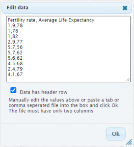
If you're getting errors on data entry, make sure that each row has data [latex]x,y[/latex] values separated with a comma. If you have the labels in the first row, make sure to select the Data has header row checkbox.
After data entry, results will be displayed on the right.
Use the options to switch variables or Show Regression Line on the graph as necessary.
y=-4.54296\colorbox{#8cf1b6}{$x$}+86.7095 = -4.54296 (\colorbox{#8cf1b6} {$3.6$}) +86.7095 = 70.3548447437 \approx 70.35
\]
y&=-4.54296x+86.7095\\
74&=-4.54296x+86.7095 &\small \textit{Plugin the value for $y$}\\
74-86.7095 &=-4.54296x &\small\textit{Subtract $86.7095$ from both sides}\\
\frac{74-86.7095}{-4.54296 } &=x &\small\textit{Divide both sides by $-4.54296$}\\
x&=2.79762558331 \approx 2.8
\end{align*}\]
Practice
Complete the practice exercise on Khan Academy: Interpreting slope and y-intercept for linear models
