
10.1 Two Population Means with Unknown Standard Deviations
HYPOTHESIS TESTING FOR DIFFERENCE BETWEEN MEANS WITH TWO SAMPLES
When testing about claims that compare two groups (populations), we'll need to obtain samples from each group to test those claims. Typically studies comparing two groups (such as the treatment and control groups in experiments/clinical trials or a company claiming that its product lasts longer than than its competitors, etc.) will require us to obtain sample from each group and use the difference between the two groups to test claim made about those populations.
Independent Samples: Two samples are independent if the selection of sample members from one population does not in any way affects the selection of sample members in the second population.
Video Example: Independent vs. Dependent Samples
In this unit, we'll perform testing using independent samples as well as depending samples. Keep in mind that the tests using independent samples follow a different procedure than that of the dependent samples.
All of hypothesis testing for means with two samples will fall into one of the following scenario:
| SCENARIO 1 |
SCENARIO 2 |
|||||
| [latex]H_0=\mu_1\ge\mu_2[/latex] [latex]H_a=\mu_1<\mu_2[/latex] |
OR | [latex]H_0=\mu_1-\mu_2\ge0[/latex] [latex]H_a=\mu_1-\mu_2 < 0[/latex] |
[latex]H_0=\mu_1\le\mu_2[/latex] [latex]H_a=\mu_1 > \mu_2[/latex] |
OR | [latex]H_0=\mu_1-\mu_2\le0[/latex] [latex]H_a=\mu_1-\mu_2 > 0[/latex] |
|
| SCENARIO 3 | ||||||
| [latex]H_0=\mu_1=\mu_2[/latex] [latex]H_a=\mu_1\ne\mu_2[/latex] |
OR | [latex]H_0=\mu_1-\mu_2=0[/latex] [latex]H_a=\mu_1-\mu_2\ne0[/latex] |
||||
Note that for scenarios 1 and 2, the null hypothesis may be written with [latex]=[/latex] sign instead of [latex]\ge[/latex] or [latex]\le[/latex].
When conducting a hypothesis test that compares two independent population means, the following characteristics should be present:
- The two independent samples are simple random samples that are independent from two distinct populations.
- If the sample sizes are small, the populations should be normally distributed. This requirement can be relaxed for larger sample sizes.
If the standard deviations of the two populations (or variances) are known, then we can conduct a [latex]z-[/latex]test to test the difference between the means. However, more often not, population standard deviations are not known. Therefore we normally do not perform this z-test. For sample sizes that are large, this test may be fine.
For the more realistic scenario when we don't know the population standard deviations, we can estimate them using the two sample standard deviations from our independent samples. If we happen to know that the population standard deviations are the same (or similar), then we can combine sample information to compute a pooled estimate of the standard deviation and use that to compute the standard error (SE), of the difference in sample means, [latex]\bar X_1-\bar X_2[/latex]: \[s_\text{pooled}=\sqrt{\frac{(n_1-1)s_1^2 +(n_2-1)s_2^2}{n_1+n_2-2}}\]
The standard error, SE: \[\text{SE}=s_\text{pooled}\sqrt{\frac{1}{n_1}+\frac{1}{n_2}}.\] The degrees of freedom, [latex]df[/latex], for the underlying [latex]t-[/latex]distribution is given by: [latex]df=n_1+n_2-2[/latex].
For situations where the population standard deviations are not known to be equal (unpooled), we calculate the estimated standard deviation, or standard error (SE), of the difference in sample means, [latex]\bar X_1-\bar X_2[/latex] as follows: \[\text{SE}=\sqrt{\frac{s_1^2}{n_1}+\frac{s_2^2}{n_2}}.\] The degrees of freedom, [latex]df[/latex], for the underlying [latex]t-[/latex] distribution is calculated either by using a conservative estimate [latex]df=\text{min}(n_1-1, n_2-1)[/latex] or by a more complicated formula, which our calculators can handle easily. \[df = \frac{\left( \frac{s_1^2}{n_1}+\frac{s_2^2}{n_2}\right)^2}{\frac{1}{n_1-1}\left(\frac{s_1^2 }{n_1} \right)^2+\frac{1}{n_2-1} \left(\frac{s_2^2 }{n_2} \right)^2}\]
You don't need to compute the gnarly formula by hand, just use a calculator. When reporting the [latex]df[/latex] computed using this formula, it doesn't always come out to be an whole number so you round down to the nearest whole number if required.
Video: To Pool or Not to Pool?
If we're comparing two populations, we may find that the population means are different. It may be due to a difference in the populations or it may be due to chance. A hypothesis test can help determine if a difference in the estimated means reflects a difference in the population means.
Generally, the null hypothesis states that the two population means are the same. That is [latex]H_0:\mu_1=\mu_2[/latex]. Recall that we start hypothesis testing by assuming the equality in the null hypothesis is true. In this case, we're assuming that [latex]\mu_1=\mu_2[/latex] which means that the two population means are the same (no difference). With no difference between the population means, we can compute the the standard deviation of the sampling distribution of the difference of the sample means as above (see both pooled and unpooled cases) and the test statistic is: \[ \frac{(\bar x_1-\bar x_2 )-(\mu_1-\mu_2)}{\sqrt{\frac{s_1^2}{n_1}+\frac{s_2^2}{n_2}}}.\] These formulas for two sample test for the difference of means are shown here so that you can recognize them for what they are but when conducting two sample tests, we'll be using calculators to speed up our calculations so that you won't have to remember these formulas.
WORKED OUT EXAMPLE - Testing with Two Samples
College Students and Drinking Habits: A public health official is studying differences in drinking habits among students at two different universities. They collect a random sample of students independently from each of the two universities and ask each student how many alcoholic drinks they consumed in the previous week. The results are summarized in the table below.
| Sample Size, [latex]n[/latex] | Sample Mean, [latex]\bar x[/latex] | Sample Standard Deviation, [latex]s[/latex] | |
| One State University | 40 | 6.9 | 2.3 |
| University of State Two | 49 | 5.7 | 1.9 |
The official wants to determine whether these data provide significant evidence that students at One State drink more than students at State Two.
SHOW SOLUTION
How can we tell?
First of all, there are two groups (or populations) that we are comparing here-- the students at two universities. We're testing to see if the average amount of drink is greater for One State. In order to do so, we'll compare the average number of drinks for each of the two groups. Since we're dealing with averages (or means), this test is going to be about means (more precisely the difference between population means). Note that since the data for each university is numerical, this points toward means as well.
Let's label One State University students' population as group 1 and University of State Two as group 2. We don't know the average number of drinks for all students at either university, so we label them as:
[latex]\mu_1[/latex] = the mean number of drinks consumed by students from One State
[latex]\mu_2[/latex] = the mean number of drinks consumed by students from State Two
Sample information
Sample information is given in table in the question.
STEP 1: Write the claim (or what's being tested) using mathematical symbols
The claim we're testing is that that students at One State drink more than students at State Two. If One State students drink less, their mean number of drinks will be lower than that of State Two students. That is, [latex]\mu_1\gt\mu_2[/latex].
STEP 2: Write the opposite of the claim using mathematical symbols
Opposite of the claim: [latex]\mu_1\le\mu_2[/latex].
STEP 3: Write the null and alternative hypothesis
The null hypothesis is the statement that contains the condition of equality which in this case is the opposite of the claim
| [latex]H_0:\mu_1\le\mu_2[/latex] [latex]H_a:\mu_1 > \mu_2[/latex] |
OR | [latex]H_0:\mu_1=\mu_2[/latex] [latex]H_a:\mu_1 > \mu_2[/latex] |
STEP 4: Identify the tail-type of the test and the level of significance, α. If α is not given, assume it to be 5% or 0.05.
This is a right tailed test. Why?
Since the level of significance is not given, use [latex]\alpha=0.05[/latex] (or 5% level of significance)
STEP 5: Check if CLT conditions are valid.
Sample sizes from both the groups are at least 30, so CLT conditions are met. We'll perform a t-test for independent means since the population standard deviations are not known.
This is the stage where we assume the equality in the null hypothesis is true, that is, assume [latex]\mu_1=\mu_2[/latex]. We're assuming that there's no difference between the two universities when it comes to their students' drinking habits. We know that the sampling distribution of the difference of sample means will be approximately normally distributed with mean of [latex]\mu_{\bar x_1-\bar x_2} = \mu_1 - \mu_2 = 0[/latex]. For the standard deviation of the sampling distribution, we need to know if the population variances are equal or unequal. If the variances are equal, then we pool their variances (POOLED), and if they are not equal, then the variances can not be pooled (NOT POOLED). In this question, we're not told that the two universities have similar variances when it comes to student drinking, so we'll proceed with an unpooled variance given by:\[\mu_{\bar x_1-\bar x_2} = \mu_1 - \mu_2 = 0 \]\[s_{\bar x_1-\bar x_2 } = \sqrt{\frac{s_1^2}{n_1}+\frac{s_2^2}{n_2}} = \sqrt{\frac{2.3^2}{40}+\frac{1.9^2}{49}}= 0.453787912342 \]
Degrees of freedom for unpooled test: \[df = \frac{\left( \frac{s_1^2}{n_1}+\frac{s_2^2}{n_2}\right)^2}{\frac{1}{n_1-1}\left(\frac{s_1^2 }{n_1} \right)^2+\frac{1}{n_2-1} \left(\frac{s_1^2 }{n_1} \right)^2}= \frac{\left( \frac{2.3^2}{40}+\frac{1.9^2}{49}\right)^2}{\frac{1}{40-1}\left(\frac{2.3^2 }{40} \right)^2+\frac{1}{49-1} \left(\frac{1.9^2}{49} \right)^2}=75.5143574829\]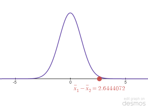
STEP 6: Plot [latex]\hat p[/latex] and find the p-value.
[latex]\bar x_1-\bar x_2[/latex] is plotted on the graph above. Since the test is right-tailed, the p-value is the area to the tail from [latex]\bar x_1-\bar x_2[/latex], shaded in purple on the graph above. To find the p-value, we can use one of the following methods:
DESMOS
✅ Find cumulative Probability (CDF)
Min: 2.64440715004 Max: [latex]\infty[/latex] (leave blank for [latex]\infty[/latex])
df can be rounded down to 75.For conservative estimate of df, use: [latex]df=\text{min}(n_1-1,n_2-1)[/latex]
[latex]=\text{min}(40-1, 49-1)=39[/latex]
STATKEY
1) Enter degrees of freedom, df
2) Select Right Tail checkbox on the top left of the graph
3) Change the value to that of our test statistic, t = 2.644 (3 decimal places)
4) The value shown in the area/proportion box at this stage is the p-value
Ti-83/84+
Enter the following, select Paste and press the ENTER button twice.
lower: 2.64440715004
upper: 10^99
df: 75.5143574829
Paste
STEP 7: Make the decision by comparing p-value with α
p-value is 0.00497452874312 which is less than [latex]\alpha[/latex] of 5%. Since p-value is less than [latex]alpha[/latex], we reject the null hypothesis ⇒ There's enough evidence to support Ha.
STEP 8: Interpret your decision in the context of original claim
The samples provide significant evidence at a significance level of 5% to conclude that students at One State drink more than students at State Two.
ONLINE CALCULATOR Approach
SUBEDI Calculator
Go to Inference for the Mean @ rsubedi.com
Input Type
Number of Samples
Independent or dependent samples?
Distribution Type for Test
Variance
For df use: Welch-Satterthwaite
Alternative Hypothesis
Confidence Interval? ← Optional
Sample Statistics Information:
| Sample Sizes | [latex]n_1:\boxed{\mathstrut\;40\;}[/latex] | [latex]n_2:\boxed{\mathstrut\;49\;}[/latex] |
| Sample Means | [latex]\bar x_1:\boxed{\mathstrut\;6.9\;}[/latex] | [latex]\bar x_1:\boxed{\mathstrut\;5.7\;}[/latex] |
| Sample Standard Deviations | [latex]s_1:\boxed{\mathstrut\;2.3\;}[/latex] | [latex]s_1:\boxed{\mathstrut\;1.9\;}[/latex] |
CALCULATE
Results show in a panel to the right. Test statistic t, p-value, and df are displayed.
LibreText Calculator
Go to: Two Independent Samples With Statistics from the list of online calculators
Enter the following values and press Calculate.
| Sample Sizes | Sample Means | Sample Standard Deviations | |
| 1st Sample | [latex]n_1:\boxed{\mathstrut\;40\;}[/latex] | [latex]\bar x_1:\boxed{\mathstrut\;6.9\;}[/latex] | [latex]s_1:\boxed{\mathstrut\;2.3\;}[/latex] |
| 2nd Sample | [latex]n_2:\boxed{\mathstrut\;49\;}[/latex] | [latex]\bar x_1:\boxed{\mathstrut\;5.7\;}[/latex] | [latex]s_1:\boxed{\mathstrut\;1.9\;}[/latex] |
|
⭕[latex]\quad\lt[/latex]
🔘[latex]\quad\gt[/latex]
⭕[latex]\quad\ne[/latex]
|
CL (confidence level) You can ignore CL entry |
CALCULATE
Results displayed are:
[latex]p[/latex]: p-value
Ignore LB and UB, if you did not enter confidence level
Example using Ti Calculator: Hypothesis Testing with Two Independent Means
Practice
