7.1 The Central Limit Theorem for Sample Means (Averages) and Proportions

SAMPLING DISTRIBUTIONS

Let’s say we are interested in knowing the average incubation period for Covid-19 virus in humans. This average is for all humans and is, therefore, a parameter, which we will label as $\mu$. Since it’s practically impossible to find out the virus incubation period for all humans and average that up to get the value of $\mu$, we will have to resort to sampling. But recall from UNIT 1 that results from random samples naturally vary from one sample to another purely due to the randomness of sampling (sampling error) which means we can’t be certain that our sample mean that we’ve calculated from our sample will always be our best estimate for the overall mean. So, our question is, how much do the sample results vary due to randomness alone? In order to investigate that, we will repeatedly and tirelessly sample from the population of our interest, compute the sample statistic of our interest from each of those samples we’ve taken, and create a histogram/dotplot of those sample results to see the shape of the distribution of the sample statistic.

In our example of the virus incubation period, let’s say we took our initial sample of 50 individuals from all over the world and recorded the incubation periods they experienced. From those 50 observations, we will calculate their average incubation period, called the sample average or the sample mean, $\overline{x}$. Let’s say first sample average was 4.5 days. Now, we’ll repeat the whole process under identical conditions by taking another random sample of 50 individuals and computing the sample mean for our second sample. Suppose the sample mean for the second sample was 5.6 days. If we repeat this process — take a sample, compute the sample mean — many times, we will obtain sample means from each of these samples:$$\begin{array}{r}{\overline{x}}_1=4.5\\ {\overline{x}}_2=5.6\\ {\overline{x}}_3=2.8\\ {\overline{x}}_4=3.4\\ \dots \\ \dots \\ \dots \end{array}$$
If we created a histogram or a dot plot of these sample means, the distribution that we’d obtain is called the sampling distribution of the sample means. Each sample mean here will be an estimator for the population mean. That is, looking at our initial sample mean of 4.5 days, our best estimate for the average virus incubation period in humans is also 4.5 days. However, if we instead take an average of all of the sample means, that average will be a better estimate of the population mean. In fact, as we add more and more sample results to find the average of the sample means, we’ll get closer and closer to the actual population mean, and this happens with just using the samples without us knowing anything about the population mean. As the number of samples increases without bound, the average of the sample means, ${\mu }_{\overline{x}}$, will equal $\mu$. Additionally, the standard deviation of these sample means, ${\sigma }_{\overline{x}}$ will equal ${\displaystyle \frac{\sigma }{\sqrt{n}}}$. The standard deviation of the sampling distribution of the sample means is also known as the standard error of the mean (SE).

The Central Limit Theorem (CLT) gives us a simple and elegant picture of what the sampling distribution of sample statistics (such as the sample mean or sample proportion) would be like given certain conditions are met. CLT is one of the most powerful and useful ideas in all of statistics.

Suppose a random variable has a mean of ${\mu }_x$ and a standard deviation of ${\sigma }_x$. For samples of size $n$ from this population, the random variable $\overline{X}$ representing sample means increasingly approximates a normal distribution as the sample size $n$ increases. $$\overline{X}\sim N({\mu }_x,\frac{{\sigma }_x}{\sqrt{n}})$$

How large should the sample size be in order for the CLT to kick in? It is generally accepted that a sample size of at least $30$ is sufficient if the population distribution unknown, with larger sample sizes providing better approximation. If the population itself is normally distributed, then the sampling distribution is normal regardless of the sample size.

EXAMPLE

The amount of coffee that people drink per day is normally distributed with a mean of $16$ ounces and a standard deviation of $6$ ounces. $18$ randomly selected people are surveyed. Round all answers to $4$ decimal places where possible.

1. What is the distribution of $X$?
2. What is the distribution of $\overline{X}$?
3. What is the probability that one randomly selected person drinks between $15.5$ and $16.5$ ounces of coffee per day?
4. For the $18$ people, find the probability that the average coffee consumption is between $15.5$ and $16.5$ ounces of coffee per day.
5. For part $(4)$, is the assumption that the distribution is normal necessary?
6. Find the IQR for the average of $18$ coffee drinkers.

SHOW SOLUTION

In this question, the random variable $X$ is the amount of coffee that people drink per day, which we’re told is normally distributed with a mean of $16$ ounces and a standard deviation of $6$ ounces.

1. $X\sim N(16,6)$.
2. $\overline{X}$ is a random variable representing sample means, and from CLT we know that the distribution of sample means is approximately normal with mean ${\mu }_{\overline{x}}=\mu$ and standard deviation ${\sigma }_{\overline{x}}={\displaystyle \frac{\sigma }{\sqrt{n}}}$. So the answer is: $\overline{X}\sim N(16,{\displaystyle \frac{6}{\sqrt{18}}}).$

ADVICE  Since the number of decimal places required is $4$ for this question, and StatKey result are to $3$ decimal places, we’ll focus on DESMOS for this question. However, StatKey method is super simple, and therefore, you may want to use StatKey first to get an idea of what the answer should be and then use DESMOS for the desired level of accuracy as needed.

DESMOS CALCULATOR
Calculator Usage Guide

3. …probability that one randomly selected person drinks between $15.5$ and $16.5$ ounces of coffee per day
In the first input box on Desmos calculator, enter: $$X=\text{normaldist}(16,6)$$ and click on the magnifying glass icon to see the normal curve. Since we want the probability/area, select the checkbox for Find Cumulative Probability (CDF) and enter 15.5 for Min, and 16.5 for Max. Area is shaded and the answer is displayed. Area/Probability $=0.0664135037052$.

4. For the $18$ people, find the probability that the average coffee consumption is between $15.5$ and $16.5$ ounces of coffee per day.
First click on the circle graph icon to the left of the input entry in the first box to turn off the graph from the last part. In the second input box on Desmos calculator, enter: $$Y=\text{normaldist}(16,6/\text{sqrt}18)$$ and click on the magnifying glass icon to see the normal curve. Since we want the probability/area, select the checkbox for Find Cumulative Probability (CDF) and enter 15.5 for Min, and 16.5 for Max. Area is shaded and the answer is displayed. Area/Probability $=0.276326390168$.

5. YES. The assumption that the population distribution is normal necessary for the CLT to work (that is for the sampling distribution of sample means to be approximately normal) here because the sample size is less than $30$.

6. …IQR for the average of $18$ coffee drinkers
Recall that to find the value given area, we need Inversecdf, and takes area to the left.
For $Q_1$: If the area to the left is 25%, then in input box #3, we enter: $$Y.\text{inversecdf}(0.25)$$ which gives us the value of $Q_1$ as $15.0461274476$.

For $Q_3$: The area to the left of $Q_3$ is 75%.
In input box #4, enter: $$Y.\text{inversecdf}(0.75)$$ Answer (displayed underneath the entry) = $16.9538725524$.
IQR = $Q_3-Q_1=1.9077451048$.

View on Desmos

Show me the steps for STATKEY

Details here!

3. …probability that one randomly selected person drinks between $15.5$ and $16.5$ ounces of coffee per day
Which distribution applies here: $X$ or $\overline{X}$ ?
We’re asked about the amount ounces of coffee per day, which is the random variable $X$. So, we’ll need to use the distribution of $X$ from part (1).
Probability that one randomly selected person drinks between $15.5$ and $16.5$ ounces of coffee per day $=P(15.5\le X\le 16.5)$
Between 15.5 and 16.5 is an interval of values of the random variable $X$. We’ll need to find the probability, which is to say we need to find the area under the curve in between 15.5 and 16.5.
On StatKey main page, click on NORMAL under Theoretical Distributions.
Click on Edit Parameters and enter your MEAN and STANDARD DEVIATION. For this question, mean $=16$ and standard deviation $=6$.
Select both Right Tail and Left Tail checkboxes at the top left. Click on the blue box below the left tail and change that to 15.5 and hit enter. Next, click on the blue box below the right tail and change that to 16.5 and hit enter. We’re looking for the area in between. Why?
Answer: 0.066. 

4. For the $18$ people, find the probability that the average coffee consumption is between $15.5$ and $16.5$ ounces of coffee per day.
Again, which distribution applies here: $X$ or $\overline{X}$ ?
Notice that in this question, we are not asked about an individual amount, but rather an average amount of daily coffee consumption for the sample of $18$ people. Because we’re asked about the sample average (sample mean), we’ll need to use the sampling distribution of sample means, $\overline{X}$.
Click on Edit Parameters and enter your MEAN and STANDARD DEVIATION for the random variable $\overline{X}$, which from part (2) is: mean $=16$ and standard deviation =$\frac{6}{\sqrt{18}}$.
Select both Right Tail and Left Tail checkboxes at the top left. Click on the blue box below the left tail and change that to 15.5 and hit enter. Next, click on the blue box below the right tail and change that to 16.5 and hit enter. We’re looking for the area in between. Answer: 0.276

5. YES. The assumption that the population distribution is normal necessary for the CLT to work (that is for the sampling distribution of sample means to be approximately normal) here because the sample size is less than $30$.

6. …IQR for the average of $18$ coffee drinkers
Once again the applicable distribution to use is that of $\overline{X}$, Why?
For IQR we need $Q_1$ and $Q_3$. Lower quartile is the location where $25$ of the values are to the left of the quartile value. So, what’s the location that has $25$ or $0.25$ of values to its left? We need to find that cut off point.
Deselect all checkboxes except the Left Tail checkbox, or make sure Left Tail is selected. Click on the blue box representing area (in the middle of the graph) and change the value to 0.25 if it is not so already. When you hit enter, the value below the number line will be your cut off point. $Q_1$: 15.046.
For $Q_3$, the area to its left will be $75$ or $0.75$. Alternatively, the area to the right of $Q_3$ will be $25$ or $0.25$. So, you can select either the left tail or right tail and supply the appropriate area to find the cut off point that will be the $Q_3$. $Q_3$: 16.954
Answer: IQR = 16.954 – 15.046  = 1.908

CLT for Sample Proportions

In our earlier example with the coronavirus, if instead we were interested in knowing the proportion of people who do not believe that Covid-19 has caused a public health crisis $(p)$, then in our sample we will be computing the sample proportion $(\hat{p}$, pronounced p-hat$)$. Sample proportion is calculated as: $\hat{p}={\displaystyle \frac{x}{n}}$, where $x=$ the number of people in the sample who do not believe that the virus has caused a health crisis, and $n$ is the sample size. If we repeat the same process of repeated sampling as with the means and draw a histogram/dot plot of sample proportions from each sample, the distribution that we’d obtain is called sampling distribution of the sample proportions. The average of sample proportions from those repeated samples will get closer and closer to the actual population proportion, ${\mu }_{\hat{p}}\to p$, and the standard deviation of the sample proportions, ${\sigma }_{\hat{p}}$ will equal $\sqrt{{\displaystyle \frac{pq}{n}}}$, where $q=1-p$. The standard deviation of the sampling distribution of sample proportions, ${\sigma }_{\hat{p}}$, is also known as the standard error of the sample proportions (SE).

EXAMPLE

A furniture company wants to know if the percent of their customers satisfied with their furniture purchase has decreased from last year’s rating of 91%. The company surveys 152 customers to gather feedback.
1. What is the distribution of $\hat{P}$?

2. What is the probability that more than 95% of those surveyed are satisfied with their purchase?

3. What is the probability that between 88% and 92% of those surveyed are satisfied with their purchase?

4. What is the range of satisfaction percentage rating that will place customer satisfaction in the middle 95% of the sampling distribution?

SHOW SOLUTION

1. We’re comparing with last year’s ratings of 91%. So, $p=0.91$. Sample size $n=152$. Since $np=138.32$ and $nq=13.68$ are both at least 5, we know from CLT that the sampling distribution of sample proportions ($\hat{p}$s) will be approximately normal with a center (mean) at ${\mu }_{\hat{p}}=0.91$ and standard deviation (std. err.) of $\sqrt{{\displaystyle \frac{p(1-p)}{n}}}=\sqrt{{\displaystyle \frac{0.91(1-0.91)}{152}}}=0.0232124059389$. The random variable $\hat{P}$ follows a normal distribution, we can write:  $\hat{P}\sim N(0.91,0.0232124059389)$.For the rest of the questions, we’ll need to use technology.

ADVICE  Since the number of decimal places required is $4$ for this question, and StatKey result are to $3$ decimal places, we’ll focus on DESMOS for this question. However, StatKey method is super simple, and therefore, you should use StatKey first to get an idea of what the answer should be and then use DESMOS for the desired level of accuracy. See previous examples for STATKEY usage.

DESMOS CALCULATOR
Calculator Usage Guide

In the first input box on Desmos calculator, enter: $$X=\text{normaldist}(0.91,0.0232124059389)$$ and click on the magnifying glass icon to see the normal curve.2. What is the probability that more than 95% of those surveyed are satisfied with their purchase?Since we want the probability/area, select the checkbox for Find Cumulative Probability (CDF) and enter 0.95 for Min. Leave the Max blank. Area is shaded and the answer is displayed. Area/Probability $=0.0424246940756$.

3. What is the probability that between 88% and 92% of those surveyed are satisfied with their purchase?
Change the Min to 0.88 and Max to 0.92 for the input boxes under Find Cumulative Probability (CDF). Area is shaded and the answer is displayed. Area/Probability $=0.568587404585$.
NOTE: Leaving Min or Max entry blank will default their values to $-\mathrm{\infty }$ and $\mathrm{\infty }$ respectively. To enter infinity $(\mathrm{\infty })$, just delete any input entered in the box and click elsewhere on the window.

4. What is the range of satisfaction percentage rating that will place customer satisfaction in the middle 95% of the sampling distribution?
Unlike in the previous two parts of the question, the 95% here refers to the area in the middle of the sampling distribution. We need to find the cut off points that separate the middle 95% of the sampling distribution of sample proportions. We use inversecdf to find cutoff points. Inversecdf takes area to the left.

If the area in the middle is 95%, then the two tail areas shaded in blue must have their areas add up to 5% which means the area of each tail is 2.5%. So the left boundary cut off point for the middle 95% has 2.5% area to its left whereas the right boundary cut off has 97.5% area to its left.

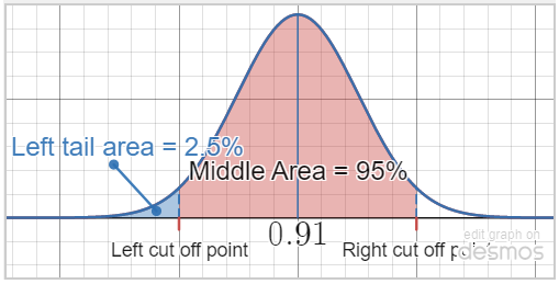Lower(Left) cut off = $X.\text{inversecdf}(0.025)=0.864504520365$ Upper(Right) cut off = $X.\text{inversecdf}(0.975)=0.955495479635$